Project activity by year
Year 1
Decide how to do traffic and vehicle simulations
TrafficSimulators_GettingStartedWithDifferrentSimulators_GettingStartedWithCARLA: Launch page to get started with CARLA (cloned from IVSG on 2023 06 05)
TrafficSimulators_GettingStartedWithDifferrentSimulators_GettingStartedWithSUMO: Launch page to get started with SUMO (cloned from IVSG on 2023 06 05)
TrafficSimulators_GettingStartedWithDifferrentSimulators_GettingStartedWithCARLA-SUMOCosimulation: Launch page to get started with CARLA-SUMO cosimulation (IVSG - PSU internal)
Mapping
About the Mapping Van
Mapping_MappingVan_About: General information about the Penn State Mapping Van. Mapping van is shown below.
Choice of Coordinate Systems for Wide Areas
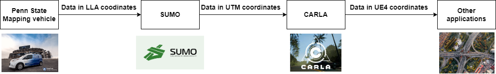
Mapping_CoordinateSystems_WideAreas: Discussion of coordinate systems and the errors each can introduce when mapping large areas (cloned from IVSG on 2023 04 03).The coordinate system conversions through simulation work are as below.
Hardware installation
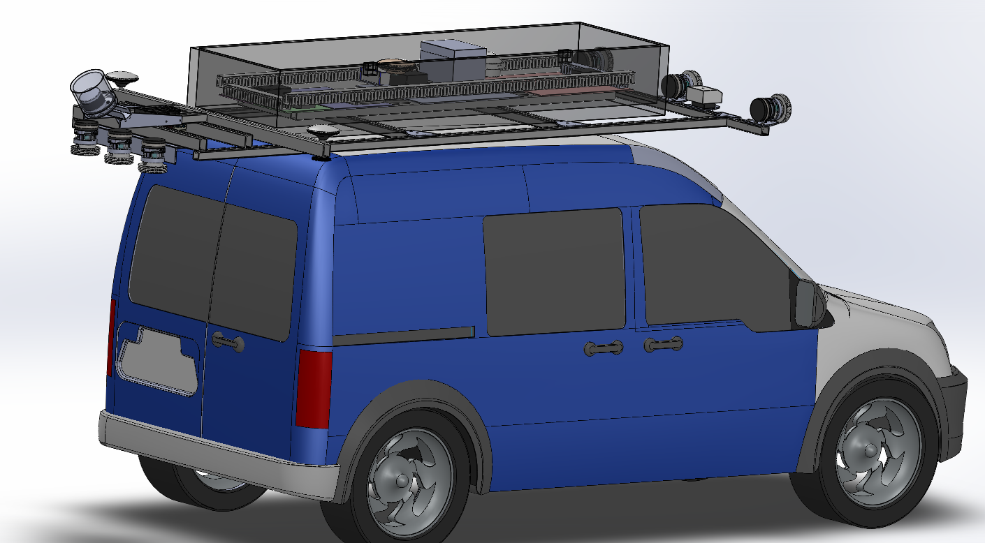
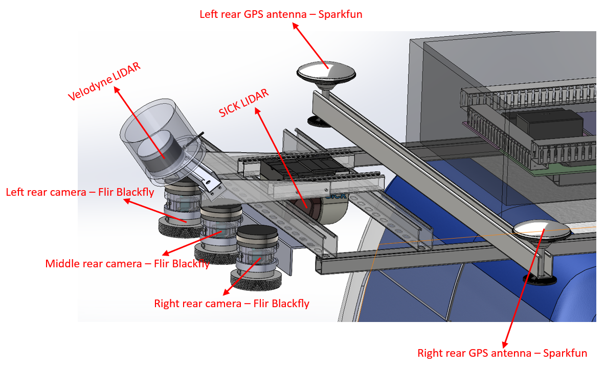
Hardware_MappingVanHardware_CADdrawings: The mapping van measurements used for the GPS antenna calibration. Sample CAD drawings are below.
Power System
Hardware_MappingVanHardware_PowerSystem: Setup of power system (IVSG - PSU internal)
Time Synchonization
FieldDataCollection_TypicalHardwareSetups_TriggerCameraUsingExternalSignal:Methods to externally trigger FLIR cameras to external trigger signals. (IVSG - PSU internal)
FieldDataCollection_TypicalHardwareSetups_TimeSync_ArduinoUsingGPSPPS: Producing tight time-trigger pulses (less than 20 microseconds jitter) via Arduinos. (IVSG - PSU internal)
FieldDataCollection_TypicalHardwareSetups_TimeSyncTriggerBox: CAD models for trigger box. (IVSG - PSU internal)
Sensors - Cameras
Hardware_MappingVanHardware_Camera: Remounting the cameras to improve regidity, water intrusion, and hardware faults. (IVSG - PSU internal)
Camera Calibration : Methods used to calibrate the camera system. (IVSG - PSU internal)
Sensors - LIDAR
Hardware_MappingVanHardware_LiDAR: Documents of LiDAR specs. (IVSG - PSU internal)
FieldDataCollection_TypicalHardwareSetups_LIDARs_CeptonX90Install: Procedure of installing CeptonX90 LiDAR. (IVSG - PSU internal)
FieldDataCollection_TypicalHardwareSetups_LIDARs_VelodyneVLP16Install: Procedure of installing VelodyneVLP16 LiDAR. (IVSG - PSU internal)
Sensors - Wheel Encoders
Hardware_MappingVanHardware_Encoder: Setup of encoders. (IVSG - PSU internal)
Sensors - Radar
Hardware_MappingVanHardware_Radar: Setup of Radar. (IVSG - PSU internal)
Sensors - GPS
Hardware_MappingVanHardware_GPS: Setup of GPS. (IVSG - PSU internal)
Sensors - IMU
Hardware_MappingVanHardware_IMU: Setup of IMU. (IVSG - PSU internal)
Sensors - Steering System
Hardware_MappingVanHardware_SteeringSystem: Setup of steering system. (IVSG - PSU internal)
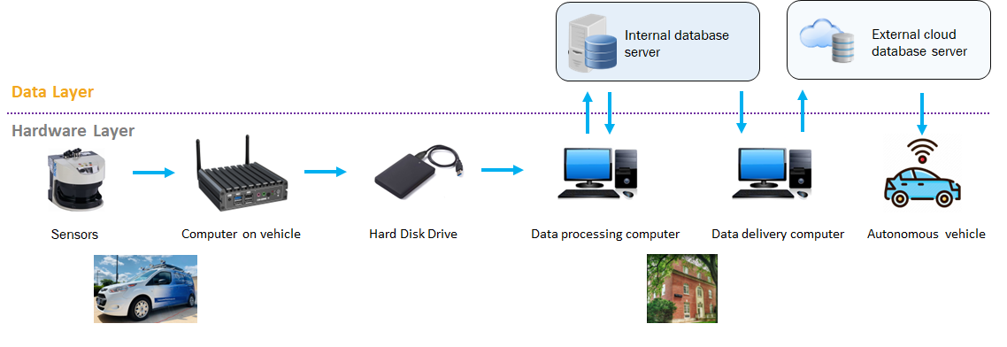
Data Parsing
FieldDataCollection_DataCollectionProcedures_ParseRawDataToDatabase: Parse raw data (.bag) to raw data database. (IVSG - PSU internal)
FieldDataCollection_DataCollectionProcedures_DataTransferWithDMS:Transfer data to PennDOT DMS. (IVSG - PSU internal)
FieldDataCollection_DataCollectionProcedures_AutomatingDataTransferToDMSUsingCommandLine: Transfer data to PennDOT DMS using command line tools. (IVSG - PSU internal)
FieldDataCollection_DataCollectionProcedures_StitchingImagesToVideo:Stitching parsed images into a video. (IVSG - PSU internal)
Year 2
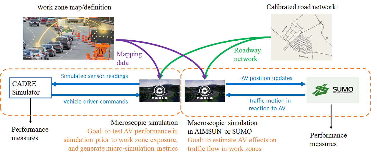
The data flow of the simulation is below
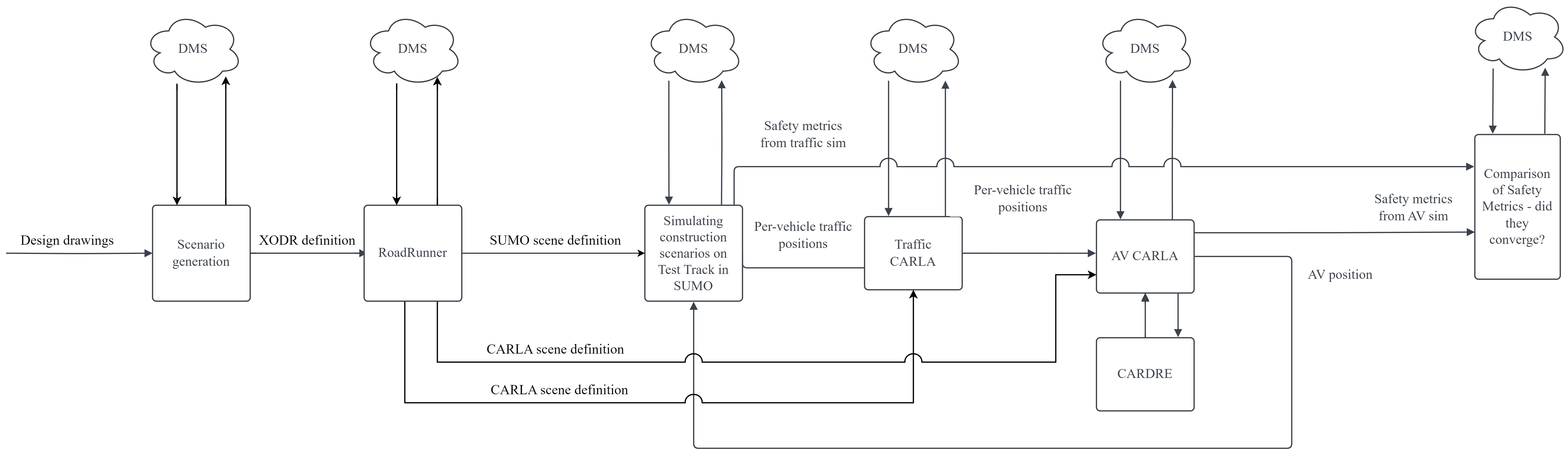
For zoomed-in view, please see: https://github.com/PAWorkzoneAutomation/PAWorkzoneAutomation.github.io/blob/main/Images/PennDOT_Simulation_Workflow_V2.drawio.png
Simulating construction scenarios
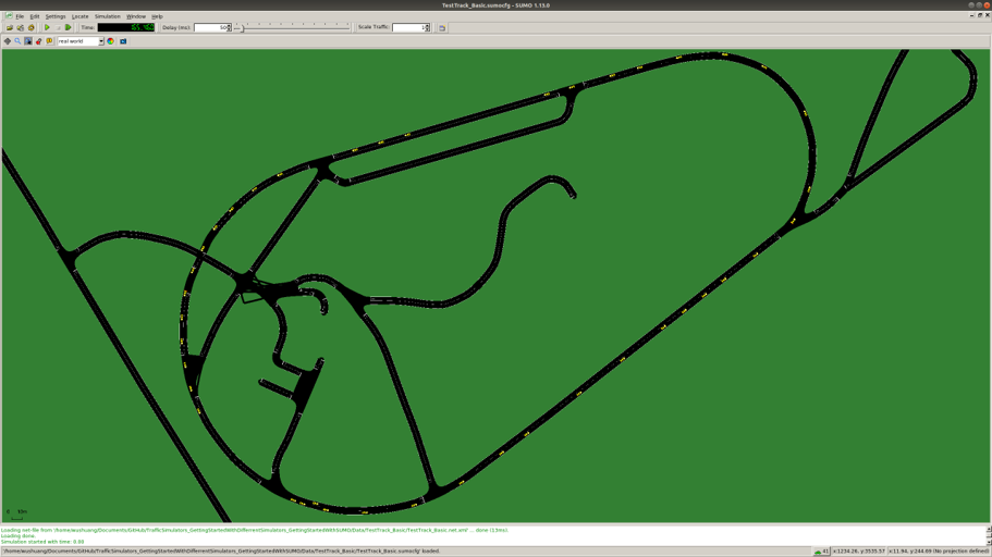
Simulating a traffic flow on Penn State test track: The work in this area involves information to guide how to simulate a traffic flow on Penn State test track. (IVSG - PSU internal)
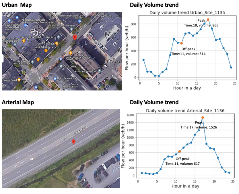
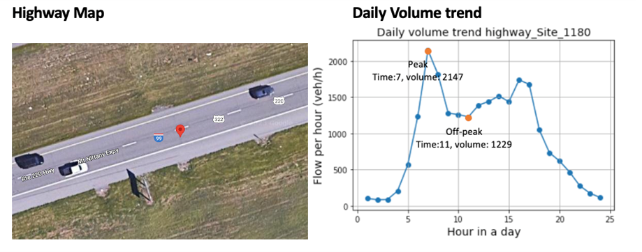
The following tables show the three roadway situations for the simulation: urban, artirial and highway, including the location we picked in State College and the corresponding data link.
Situations |
Urban |
|---|---|
City |
PA, State College |
Location Description |
|
Site Number |
1134 |
Data Time |
Nov 16, 2016 |
Peak Time |
8AM |
Peak Volume (Vehicles/h) |
696 |
Off-peak Time |
1PM |
Off-peak Volume (Vehicles/h) |
368 |
Link to Real Traffic Data |
Situations |
Arterial |
|---|---|
City |
PA, State College |
Location Description |
|
Site Number |
1136 |
Data Time |
Nov 16, 2016 |
Peak Time |
5PM |
Peak Volume (Vehicles/h) |
2374 |
Off-peak Time |
9AM |
Off-peak Volume (Vehicles/h) |
1212 |
Link to Real Traffic Data |
Situations |
Highway |
|---|---|
City |
PA, State College |
Location Description |
|
Site Number |
1180 |
Data Time |
Dec 05, 2017 |
Peak Time |
4PM |
Peak Volume (Vehicles/h) |
4046 |
Off-peak Time |
9AM |
Off-peak Volume (Vehicles/h) |
2321 |
Link to Real Traffic Data |
The following table shows the summary about whether the considered three roadway situations could be applied to each of the proposed 20 scenarios.
Scenario |
Scenario Summary |
Urban |
Arterial |
Highway |
Uploaded to DMS |
|---|---|---|---|---|---|
0 |
ANALYSIS OF VARIANCE |
Y |
Y |
Y |
Urban peak volume Urban off-peak volume Arterial peak volume Arterial off-peak volume |
1.1 |
|
Y |
Y |
Y |
Urban peak volume |
1.2 |
|
Y |
Y |
Y |
|
1.3 |
|
N |
N |
Y |
|
1.4 |
|
N |
N |
Y |
|
1.5 |
|
Y |
Y |
N |
|
1.6 |
|
N |
N |
Y |
|
2.1 |
|
Y |
Y |
Y |
|
2.2 |
|
Y |
Y |
Y |
|
2.3 |
LANE SHIFT TO TEMPORARY ROADWAY |
Y |
Y |
Y |
|
2.4 |
|
Y |
Y |
Y |
|
3.1 |
|
Y |
Y |
Y |
|
4.1a |
|
Y |
Y |
Y |
|
4.1b |
|
N |
N |
Y |
|
4.2 |
|
N |
N |
Y |
|
4.3 |
|
N |
N |
Y |
|
5.1a |
|
Y |
Y |
Y |
|
5.1b |
|
N |
N |
Y |
|
5.2 |
|
Y |
Y |
Y |
|
6.1 |
|
Y |
Y |
Y |
Variance analysis of simulation results
The daily volume trends of urban, arterial and highway are summarized below:
We did an analysis of variance to check whether simulated flow is the same as the set flow and to find the minimum simulation time.
The flow is estimated every 1 min. The data used below is right from the peak start time or off-peak start time, from the detector on the test track for two lanes.
The results are shown as below.
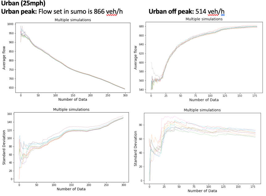
Results for urban
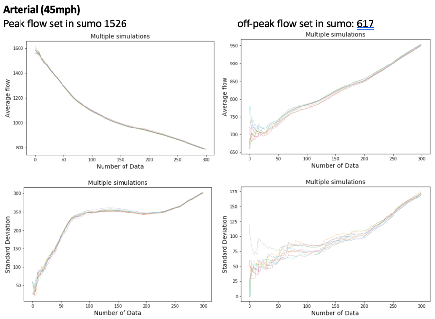
Results for arterial
Analysis for highway is ongoing.
Simulation post processing
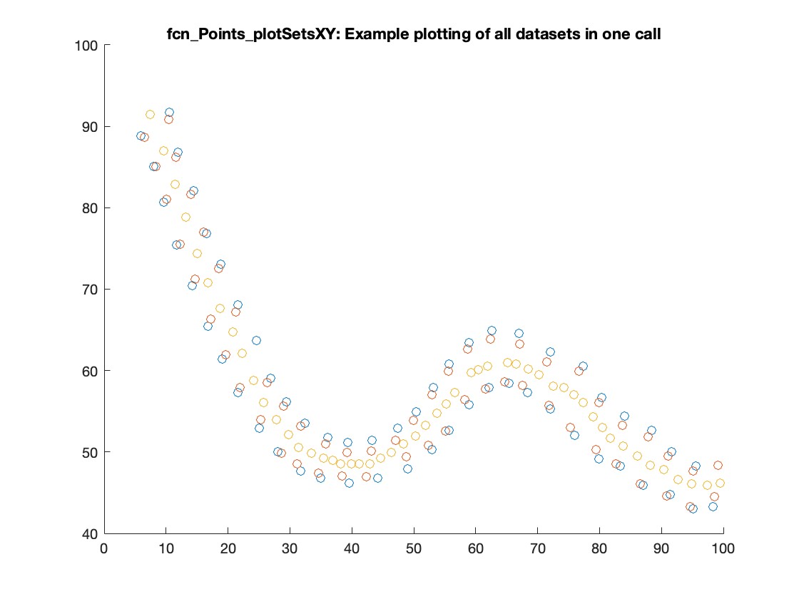
FeatureExtraction_Association_PointToPointAssociation: Functions are provided to determine matches between data sets of (X,Y) points, store and compare groups of associated points (patch objects), and determine intersections between patch objects and circular arcs (useful for collision detection).
FeatureExtraction_SafetyMetrics_SafetyMetricsClass: MATLAB code implementation of functions that perform safety metric calculations given a set of objects and a path through them.
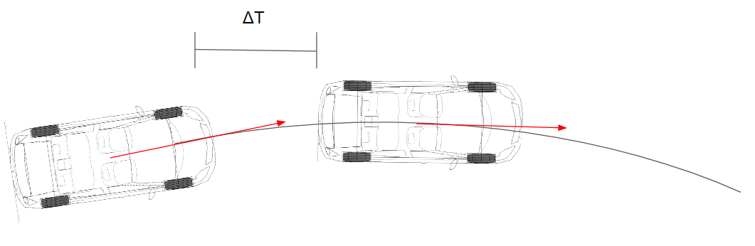
Time to collision
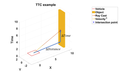
Example of TTC calculation
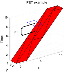
Example of PET calculation
Demo of vehicle doing a lane change
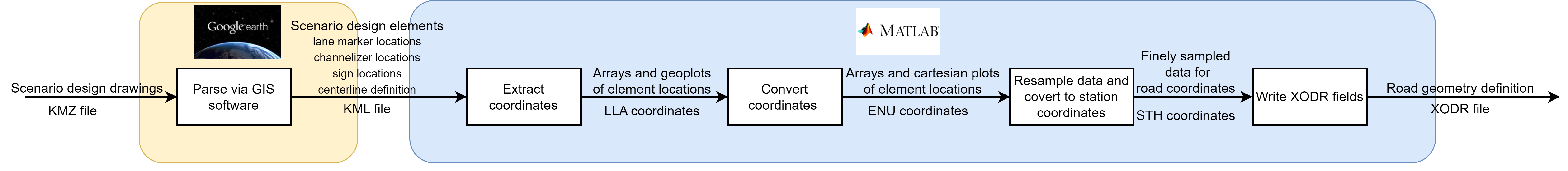
Automatic generation of work zone simulation scenarios
The automatic generation of scenarios for simulation that follow the workflow as below:
The source file of this workflow diagram can be found here: https://drive.google.com/file/d/18G0Bb3WNbk9Mf6DgM548p8j4xtOKnf1m/view?usp=sharing
Scenarios defined in KMZ format are loaded into GIS software, such as Google Earth.
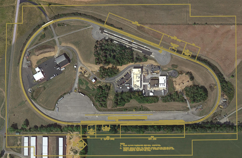
This contains all data for the CAD definition, but most of this is not needed within final road definition as per ASAM OpenDRIVE.
The KMZ files can be found here: https://github.com/ivsg-psu/FieldDataCollection_VisualizingFieldData_PlotWorkZone/tree/main (IVSG internal)
The KMZ definition is then parsed to KML, where coordinates are readable.
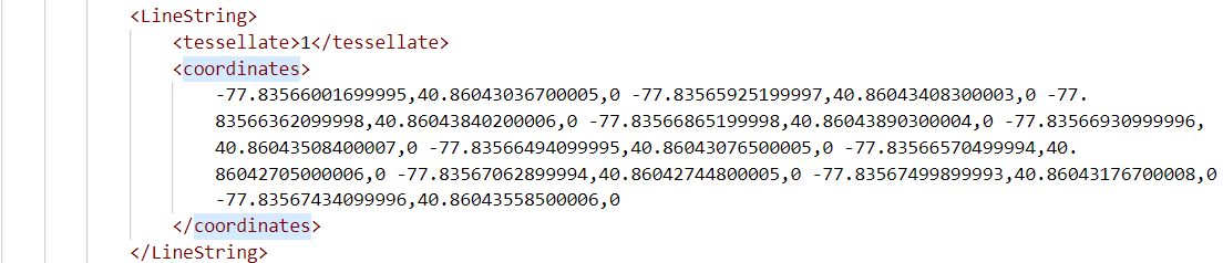
The KML files can be found here: https://github.com/ivsg-psu/FieldDataCollection_VisualizingFieldData_PlotWorkZone/tree/main (IVSG internal)
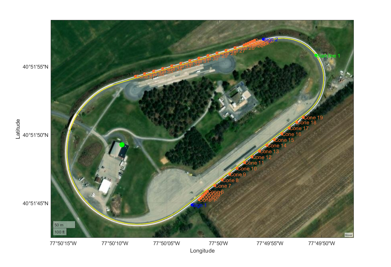
The KML definition is parsed in MATLAB. It illustrates driving lanes and traffic objects in LLA coordinate system.
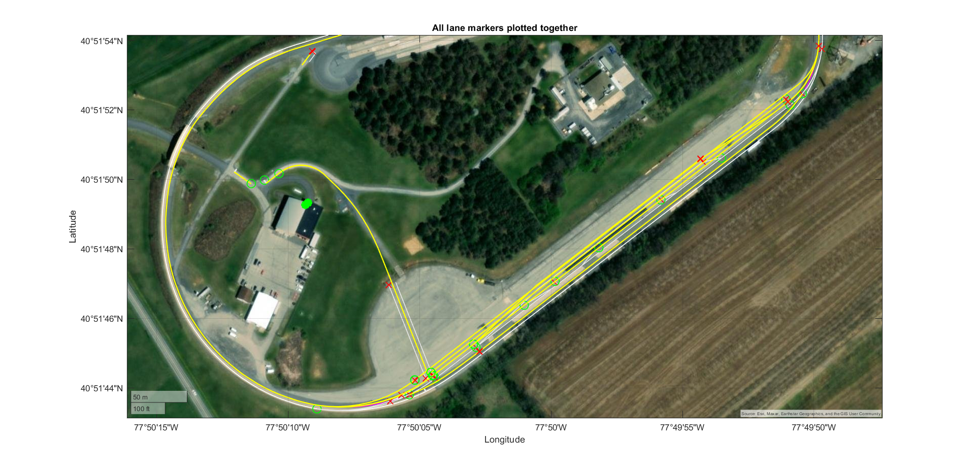
Using the KML data, we can plot all the scenarios with each other to identify common lane markers and road segments.
The driving lanes in LLA coordinates are then transformed into ENU coordinates. This uses the Cartesian coordinates to ease the creation of XODR definitions.
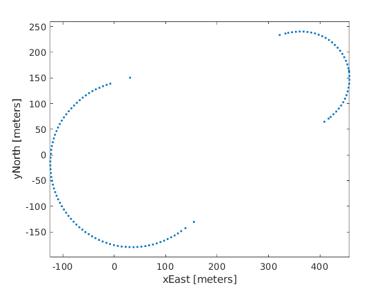
Non-smooth data points contain large gaps, and this causes problems when the road is created.
Example of test track created with non-smooth data points
Problem of misalignment caused by the non-smooth data points
The ENU coordinates are then resampled for geometric smoothness to avoid the large gaps
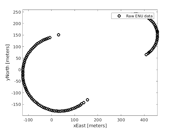
Raw ENU data of test track
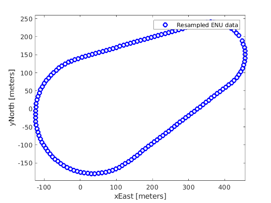
resampled ENU data of test track
The resampled ENU coordinates are then converted to XODR definition.
The xodr file can be found as testTrack.xodr with this link: https://github.com/PAWorkzoneAutomation/PAWorkzoneAutomation.github.io/tree/main/Data/MapImports/XODR
The XODR file is then editable to apply to different scenarios, for example, changing the lane width. Below shows an example of increasing the right driving lane width.
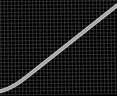
Original |

Lane width increased |
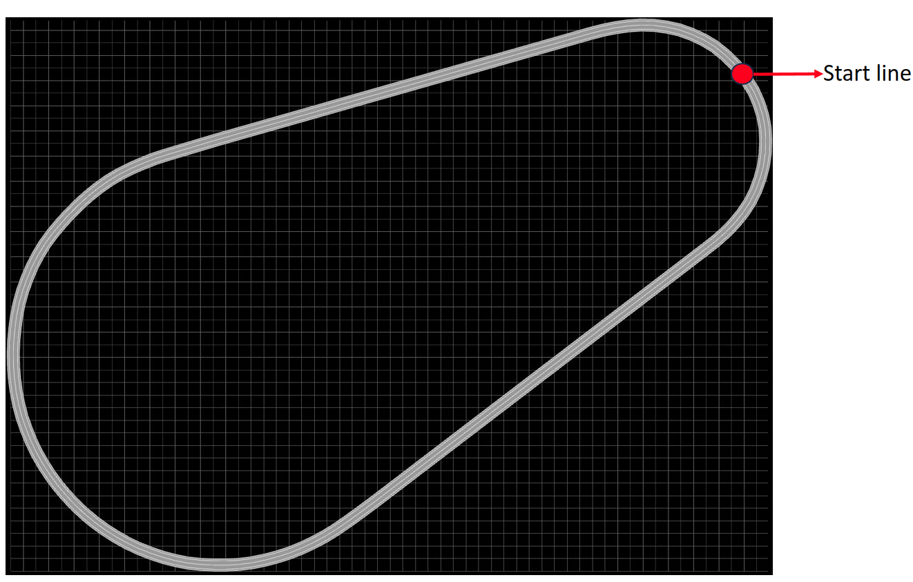
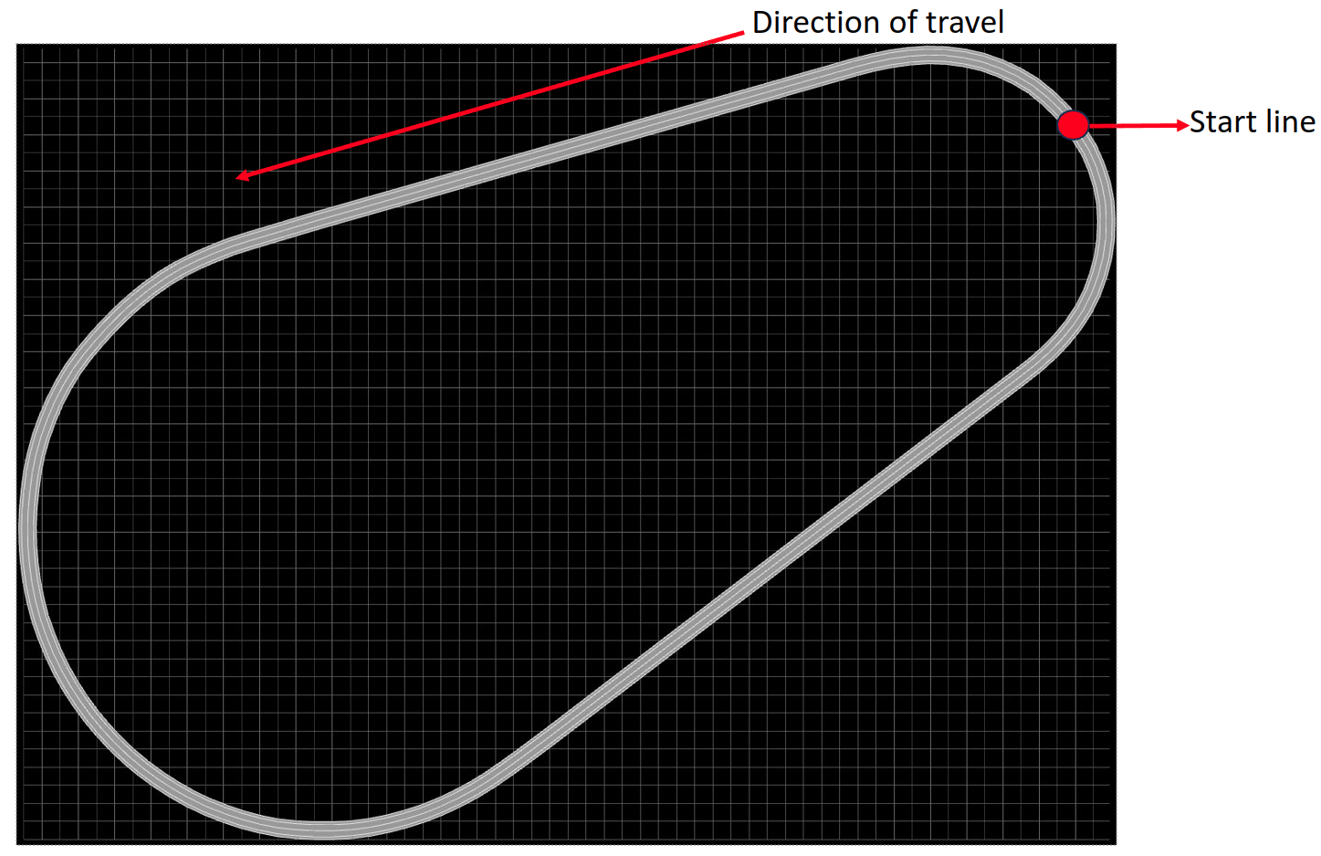
Below shows another example of increasing the right driving lane width at 500 meters from the start line.

The xodr file can be found as testTrack_increasedLaneWidth.xodr with this link: https://github.com/PAWorkzoneAutomation/PAWorkzoneAutomation.github.io/tree/main/Data/MapImports/XODR
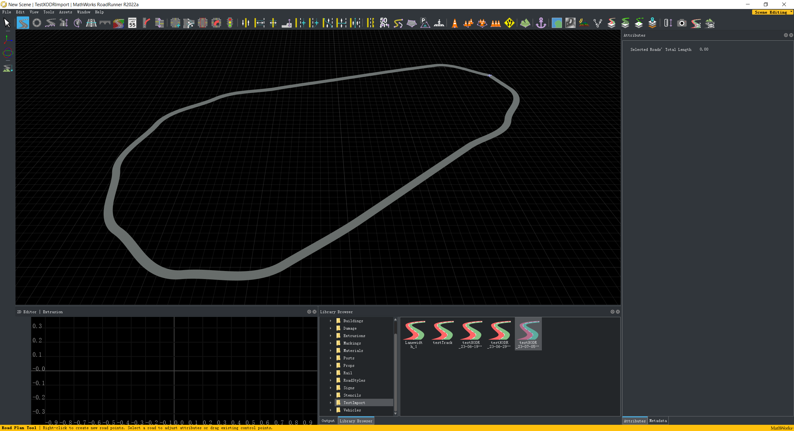
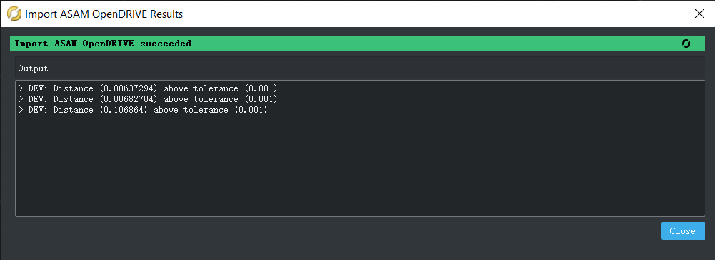
XODR can be imported into RoadRunner.
Road imported into XODR viewer (open-source) |
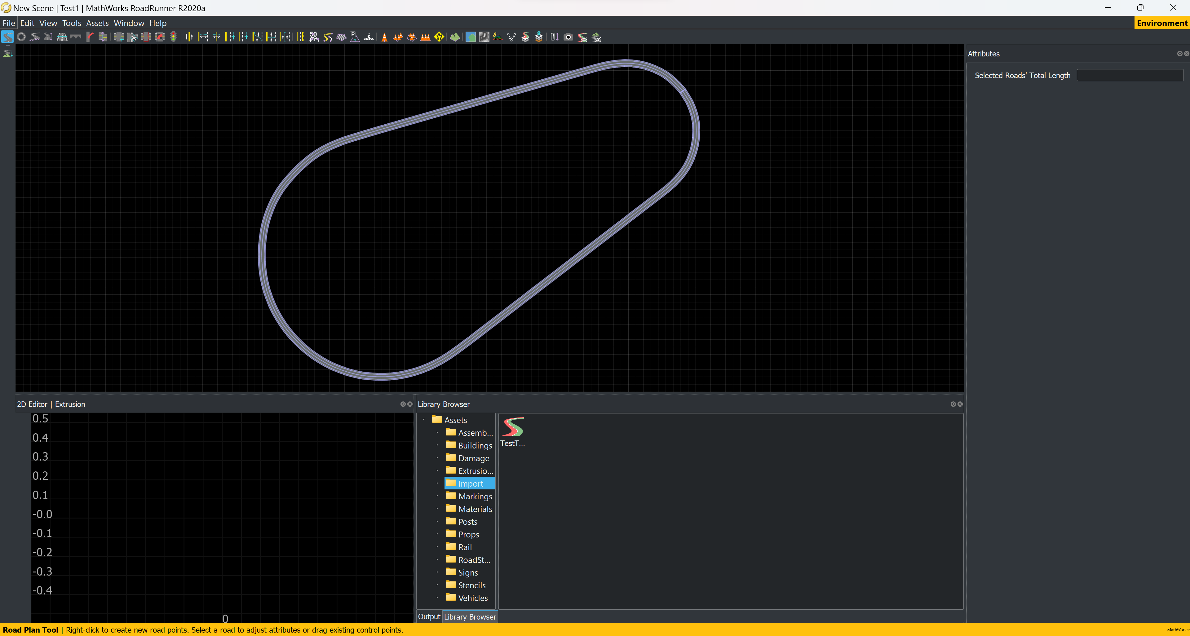
Road imported into RoadRunner (commercial) |
The xodr file can be found as testTrack.xodr with this link: https://github.com/PAWorkzoneAutomation/PAWorkzoneAutomation.github.io/tree/main/Data/MapImports/XODR
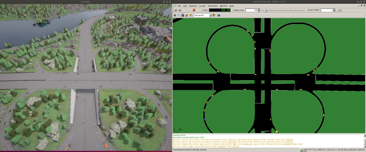
RoadRunner exports into CARLA and SUMO.
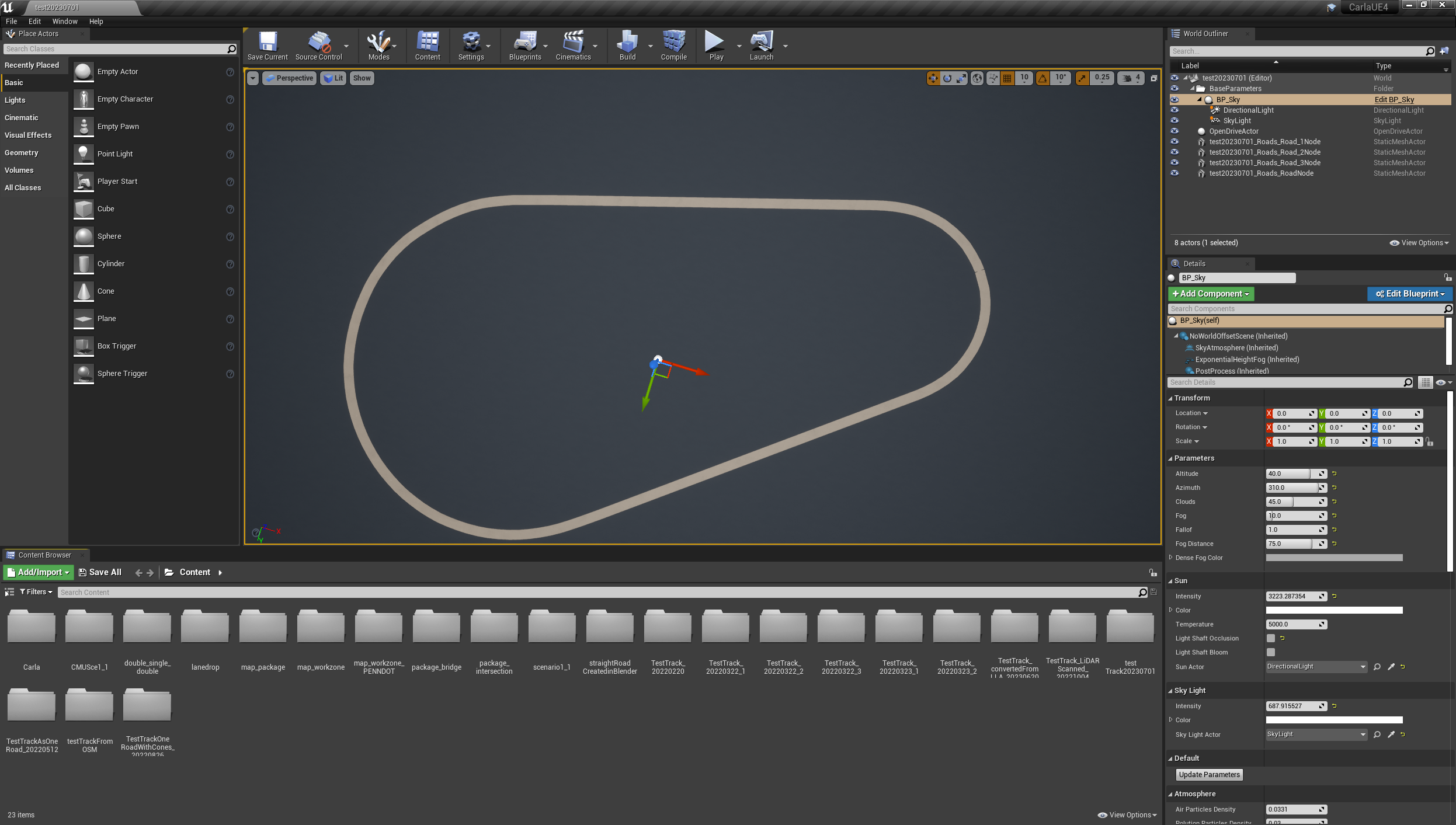
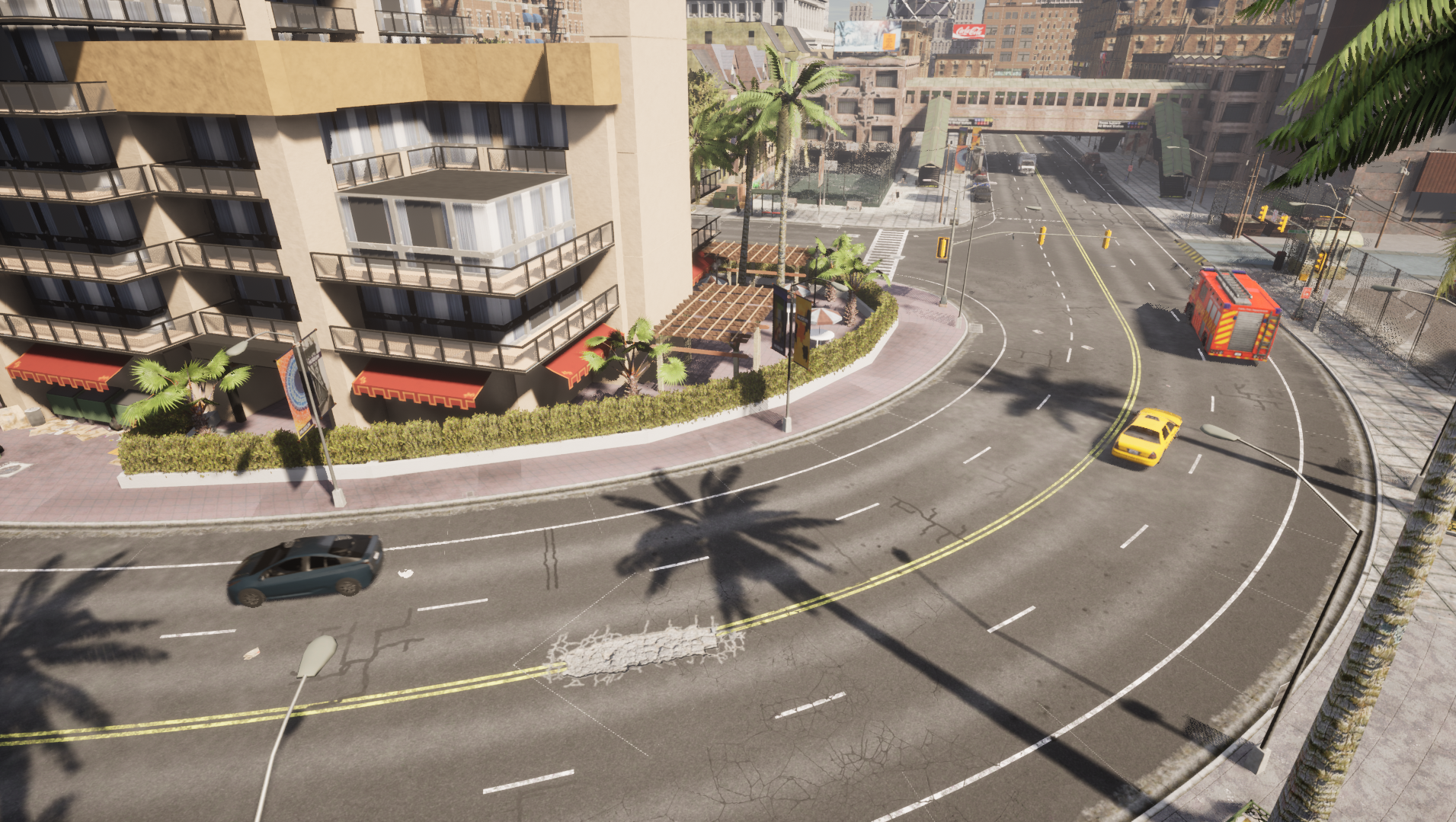
Test track imported into CARLA |
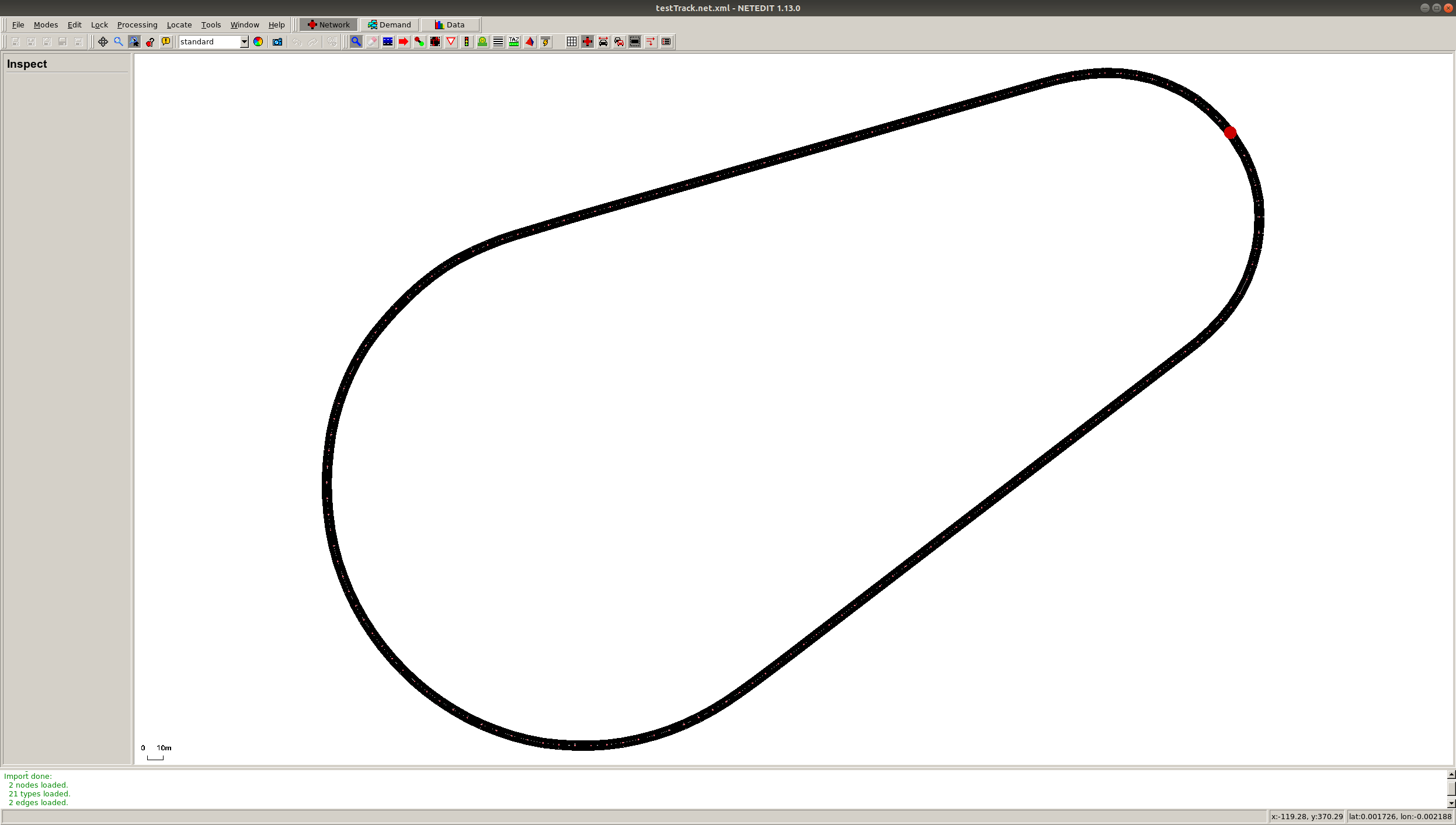
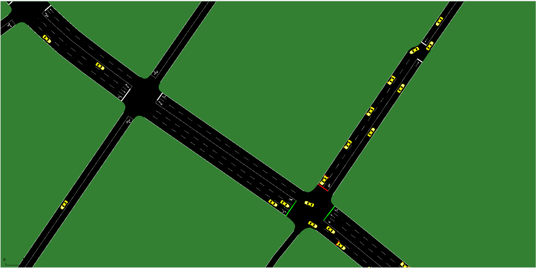
Test track imported into SUMO |
The files needed for map imports can be found with this link: https://github.com/PAWorkzoneAutomation/PAWorkzoneAutomation.github.io/tree/main/Data/MapImports
Year 3
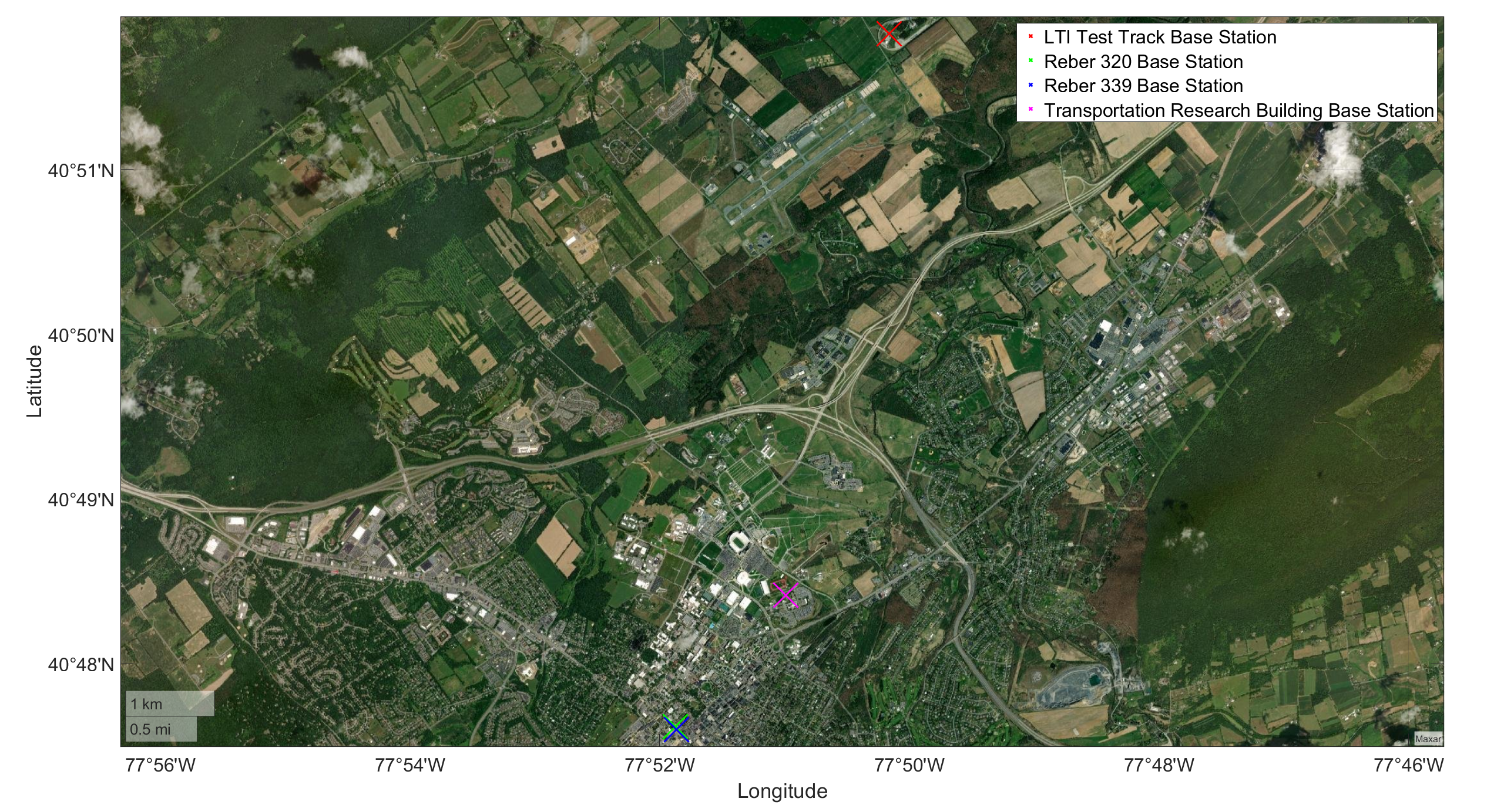
GPS and CORS Calibration
FieldDataCollection_GPSRelatedCodes_RTKCorrectionService: Setting up and using of Real-time kinematic (RTK) via Networked Transport of RTCM via Internet Protocol (NTRIP).(IVSG - PSU internal).
Name |
Server ID |
Base Station LLA Coordinates |
Datumn |
Installation Date |
Last Calibration Date |
Note |
|---|---|---|---|---|---|---|
LTI Test Track Base Station |
PSU_TestTrack |
TBD |
WGS 84 |
TBD |
TBD |
Installed and maintained by IVSG. |
Reber 320 Base Station |
PSU_Reber320 |
40.79365087° -77.86460284° 334.719 m |
WGS 84 |
11/28/2022 |
01/07/2023 |
Installed and maintained by IVSG, this base station is moveable so it cannot be used as a CORS station |
Reber 339 Base Station |
PSU_Reber339 |
40.79333290° -77.86441976° 334.733 m |
WGS 84 |
11/28/2022 |
01/08/2023 |
Installed and maintained by IVSG, this base station is moveable so it cannot be used as a CORS station |
Transportation Research Building Base Station |
PSU1 |
40.8068919389° -77.8497968306° 337.665 m |
WGS 84 |
TBD |
TBD |
Installed and maintained by PennDOT, its LLA coordinates may not be correct. |
Data Processing
Processing GPS Data
DataProcessing_GPS_GPSConversionMethods: A repo sharing the algorithms used for GPS conversions, e.g. LLA to ENU (cloned from IVSG on 2023 04 03).
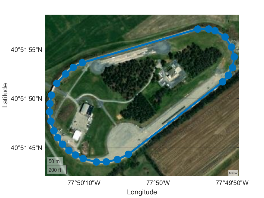
Example of LLA data collected
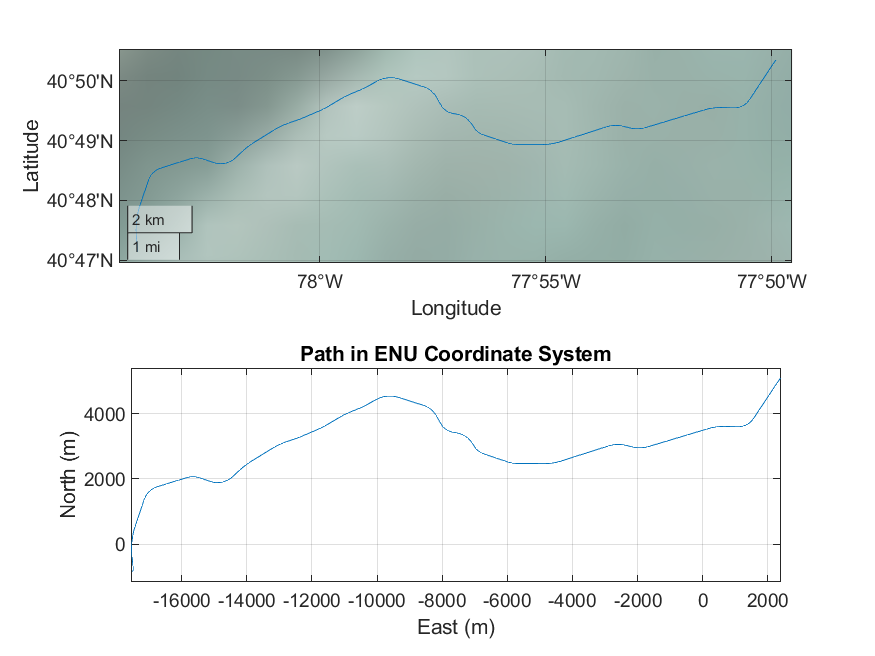
Example of LLA data converted to ENU
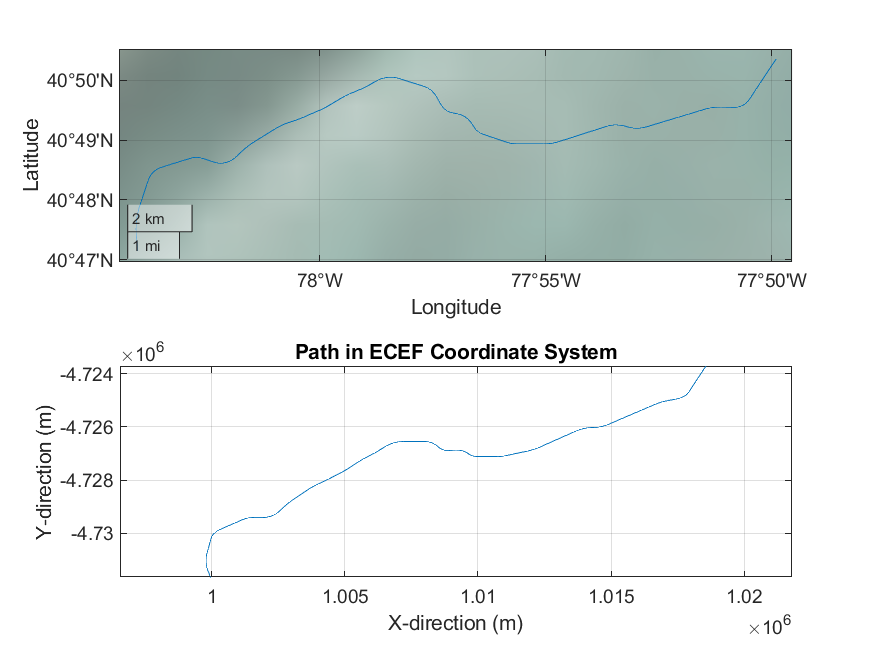
Example of LLA data converted to ECEF
FeatureExtraction_DataTransforms_TransformClassLibrary: A repo contains transformation operations typically needed for cartesian data processing.
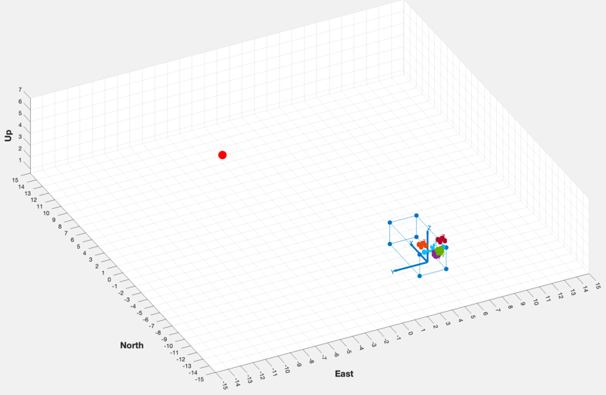
Example of transforming sensor reading from the ENU coordinates to sensor coordinates
Maps and scenarios
FieldDataCollection_VisualizingFieldData_PlotWorkZone: A repo displaying the scenarios and their descriptions. (IVSG - PSU internal)
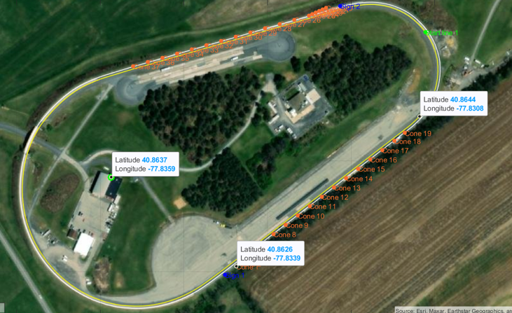
Example of lane markers and traffic objects for scenario 1.1
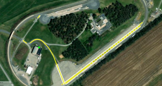
Plot of all lane markers to be painted on the test track (as per their color and type)
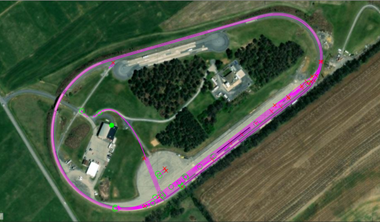
Plot of all lane markers needed to complete 19 scenarios (overlapping)
Data collection for on-track tests
Year 4
Set up work zone in live on-road
Map work zone in live on-road
Process/Upload map
Conduct live on-road testing
Collect/Process/Upload/Analyze live on-road testing data